V.II.1
Univariate Transfer Function Identification
A
relationship between two variables under investigation may be linear
or nonlinear. Sometimes it is possible to transform a
nonlinear relationship into a linear one by use of power
transformations.
We
may identify nonlinearities by using half-slopes. First we
partition the observations of a scatter plot into three equal parts
(each part consisting of approximately the same amount of
observations). Then we compute the medians of each partition
yielding a set of three pairs of coordinates:

The
half-slopes are computed by

(V.II.1-1)
whereas
the half-slope ratio is

(V.II.1-2)
If
this ratio is equal to 1, no transformation is required. On the
other hand, if
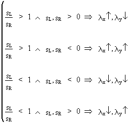
(V.II.1-3)

Remark
that if the ratio is negative, no power transformation can be used
to linearize the relationship.
The
dependence between the input variable (c.q. the exogenous variable),
and the output variable (c.q. the endogenous variable) must not be
restricted to linear models. Let us therefore have a closer look at
the so-called impulse response function (IRF). A simple
example of an IRF is

(V.II.1-4)

In
order to have the transfer function allow only finite incremental
changes in the output series (if the input series undergoes a finite
change), the model must be checked for stability.


(V.II.1-5)
is
called the steady gain of the model. Note that this gain converges
in stable models.
On
using the more general (and parsimonious) formulation of the pure
(c.q. without noise) transfer function model

(V.II.1-6)


(V.II.1-7)
This
result can be used to obtain
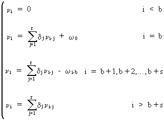
(V.II.1-8)

Obviously
a transfer function model depends on the parameters r, s, and b
(c.q. TF(r,s,b)). Hence, on using (V.II.1-8), for any TF(r,s,b)
model the theoretical impulse-response function can be obtained. A
likewise procedure can be used to obtain the step impulse functions
for any TF(r,s,b) model.
If
one is concerned with identifying a transfer function relationship
between the input and output variable, and if the input variable is
not a white noise series, a prewhitening step should precede
the computation of a cross correlation function (CCF). In order to
see this, consider the identification of the impulse response
function without prewhitening (c.q. when the input series is not
white noise).
If
W(t), X(t), and N(t) are stationary series then the impulse response
function

(V.II.1-9)


(V.II.1-10)
On
assuming that the input variable, and N(t) are uncorrelated; and on
taking expectations, the covariance function is obtained

(V.II.1-11)
from
which it can be seen that a relationship exists between the
impulse-response function and the covariance function. If however
the input X(t) is not white noise, the cross covariance function
(and hence also the CCF) is distorted due to autocorrelation, since
(V.II.1-10) becomes
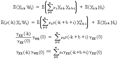
(V.II.1-12)
where
it is implicitly assumed that X(t) is uncorrelated with N(t); W(t),
and X(t) are stationary (though autocorrelated) time series with
zero mean; and k = 0, 1, 2, ...
In
order to compute the prewhitened cross correlation function (PCCF),
we first filter the stationary input variable X(t) through its
univariate stochastic (ARIMA) model

(V.II.1-13)
such
that the white noise series a(t)
is obtained. Second, the stationary output series Y(t) is
transformed through the same filter

(V.II.1-14)
from
which it can be deduced that
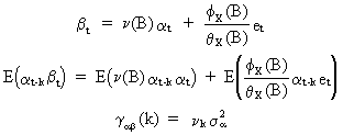
(V.II.1-15)


(V.II.1-16)
where
in practice the estimated standard errors and correlation
coefficients are used.

Thus,
the PCCF can be used for transfer function identification purposes:


-
the residual ACF and PACF (of the transfer function model) can be
used for checking purposes, and provides a mean to adapt
inadequately identified models.
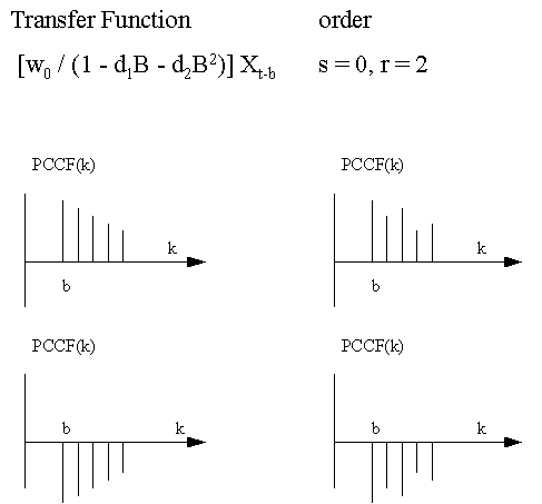
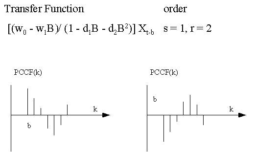
This
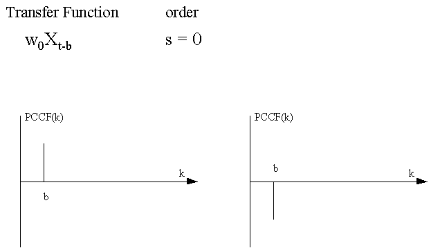
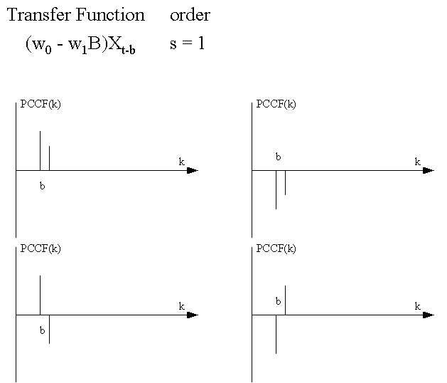
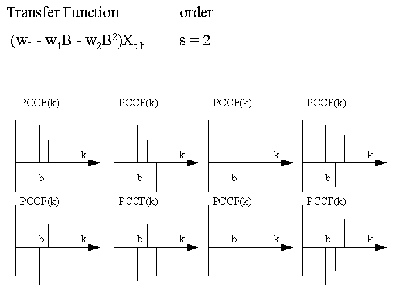
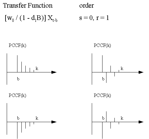
is a graphical summary of various types of Transfer Function-Noise
models that can be identified by the use of the PCCF:
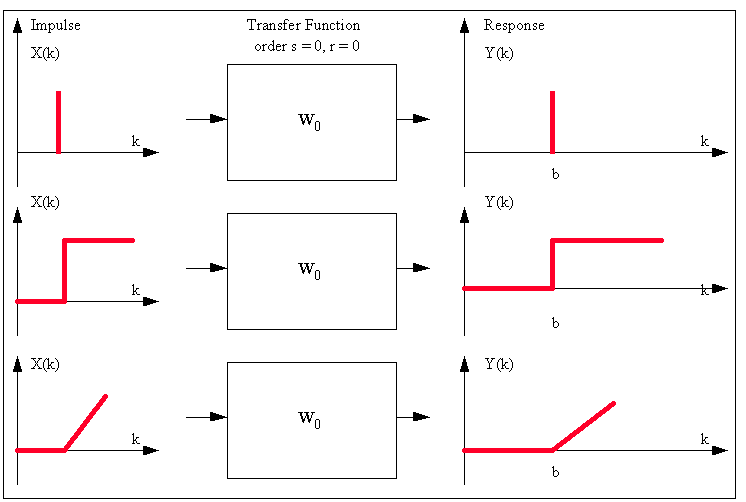
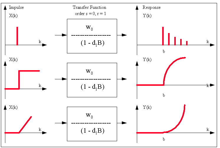
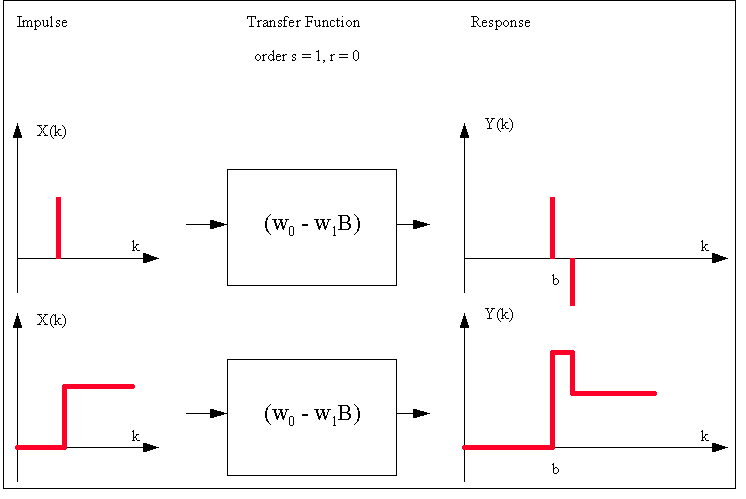
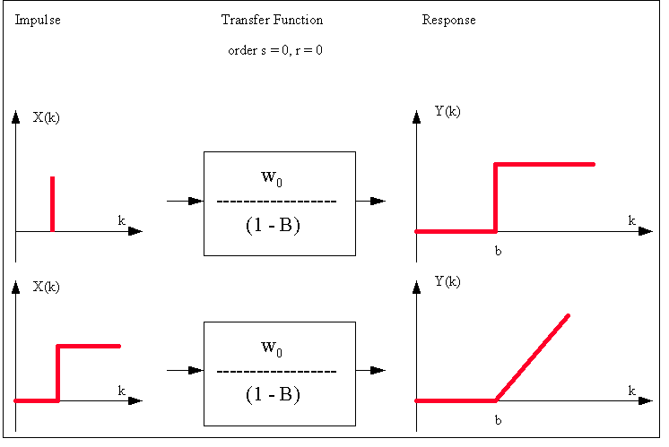
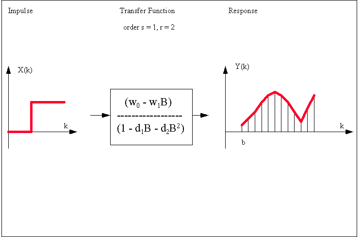
This
is a graphical summary of various types of Impulse Response
Functions that can be investigated:
| 
